Parallel stream processing with zero-copy fan-out and sharding

In a previous post I explored how we can make better use of our parallel hardware by means of pipelining.

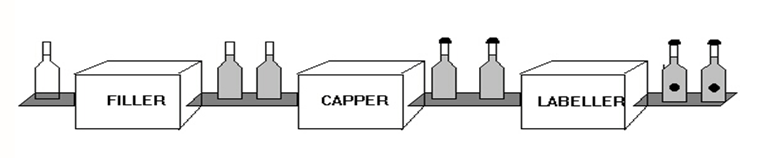
In a nutshell the idea of pipelining is to break up the problem in stages and have one (or more) thread(s) per stage and then connect the stages with queues. For example, imagine a service where we read some request from a socket, parse it, validate, update our state and construct a response, serialise the response and send it back over the socket. These are six distinct stages and we could create a pipeline with six CPUs/cores each working on a their own stage and feeding the output to the queue of the next stage. If one stage is slow we can shard the input, e.g. even requests to go to one worker and odd requests go to another thereby nearly doubling the throughput for that stage.

One of the concluding remarks to the previous post is that we can gain even more performance by using a better implementation of queues, e.g. the LMAX Disruptor.

The Disruptor is a low-latency high-throughput queue implementation with support for multi-cast (many consumers can in parallel process the same event), batching (both on producer and consumer side), back-pressure, sharding (for scalability) and dependencies between consumers.

In this post we’ll recall the problem of using “normal” queues, discuss how Disruptor helps solve this problem and have a look at how we can we provide a declarative high-level language for expressing pipelines backed by Disruptors where all low-level details are hidden away from the user of the library. We’ll also have a look at how we can monitor and visualise such pipelines for debugging and performance troubleshooting purposes.

Motivation and inspiration

Before we dive into how we can achieve this, let’s start with the question of why I’d like to do it.

I believe the way we write programs for multiprocessor networks, i.e. multiple connected computers each with multiple CPUs/cores, can be improved upon. Instead of focusing on the pitfalls of the current mainstream approaches to these problems, let’s have a look at what to me seems like the most promising way forward.

Jim Gray gave a great explanation of dataflow programming in this Turing Award Recipient interview. He uses props to make his point, which makes it a bit difficult to summaries in text here. I highly recommend watching the video clip, the relevant part is only three minutes long.

The key point is exactly that of pipelining. Each stage is running on a CPU/core, this program is completely sequential, but by connecting several stages we create a parallel pipeline. Further parallelism (what Jim calls partitioned parallelism) can be gained by partitioning the inputs, by say odd and even sequence number, and feeding one half of the inputs to one copy of the pipeline and the other half to another copy, thereby almost doubling the throughput. Jim calls this a “natural” way to achieve parallelism.

While I’m not sure if “natural” is the best word, I do agree that it’s a nice way to make good use of CPUs/cores on a single computer without introducing non-determinism. Pipelining is also effectively used to achieve parallelism in manufacturing and hardware, perhaps that’s why Jim calls it “natural”?

Things get a bit more tricky if we want to involve more computers. Part of the reason, I believe, is that we run into the problem highlighted by Barbara Liskov at the very end of her Turing award lecture (2009):

“There’s a funny disconnect in how we write distributed programs. You write your individual modules, but then when you want to connect them together you’re out of the programming language and into this other world. Maybe we need languages that are a little bit more complete now, so that we can write the whole thing in the language.”

Ideally we’d like our pipelines to seamlessly span over multiple computers. In fact it should be possible to deploy same pipeline to different configurations of processors without changing the pipeline code (nor having to add any networking related code).

A pipeline that is redeployed with additional CPUs or computers might or might not scale, it depends on whether it makes sense to partition the input of a stage further or if perhaps the introduction of an additional computer merely adds more overhead. How exactly the pipeline is best spread over the available computers and CPUs/cores will require some combination of domain knowledge, measurement and judgment. Depending on how quick we can make redeploying of pipelines, it might be possible to autoscale them using a program that monitors the queue lengths.

Also related to redeploying, but even more important than autoscaling, are upgrades of pipelines. That’s both upgrading the code running at the individual stages, as well as how the stages are connected to each other, i.e. the pipeline itself.

Martin Thompson has given many talks which echo the general ideas of Jim and Barbara. If you prefer reading then you can also have a look at the reactive manifesto which he cowrote. Martin is also one of the people behind the Disruptor, which we will come back to soon, and he also said the following:

“If there’s one thing I’d say to the Erlang folks, it’s you got the stuff right from a high-level, but you need to invest in your messaging infrastructure so it’s super fast, super efficient and obeys all the right properties to let this stuff work really well.”

This quote together with Joe Armstrong’s anecdote of an unmodified Erlang program only running 33 times faster on a 64 core machine, rather than 64 times faster as per the Ericsson higher-up’s expectations, inspired me to think about how one can improve upon the already excellent work that Erlang is doing in this space.

Longer term, I like to think of pipelines spanning computers as a building block for what Barbara calls a “substrate for distributed systems”. Unlike Barbara I don’t think this substrate should be based on shared memory, but overall I agree with her goal of making it easier to program distributed systems by providing generic building blocks.

Prior work

Working with streams of data is common. The reason for this is that it’s a nice abstraction when dealing with data that cannot fit in memory. The alternative is to manually load chunks of data one wants to process into memory, load the next chunk etc, when we processes streams this is hidden away from us.

Parallelism is a related problem, in that when one has big volumes of data it’s also common to care about performance and how we can utilise multiple processors.

Since dealing with limited memory and multiprocessors is a problem that as bothered programmers and computer scientists for a long time, at least since the 1960s, there’s a lot of work that has been done in this area. I’m at best familiar with a small fraction of this work, so please bear with me but also do let me know if I missed any important development.

In 1963 Melvin Conway proposed coroutines, which allows the user to conveniently process very large, or even infinite, lists of items without first loading the list into memory, i.e. streaming.

Shortly after, in 1965, Peter Landin introduced streams as a functional analogue of Melvin’s imperative coroutines.

A more radical departure from Von Neumann style sequential programming can be seen in the work on dataflow programming in general and especially in Paul Morrison’s flow-based programming (late 1960s). Paul uses the following picture to illustrate the similarity between flow-based programming and an assembly line in manufacturing:

Each stage is its own process running in parallel with the other stages. In flow-based programming stages are computation and the conveyor belts are queues. This gives us implicit parallelism and determinate outcome.

Doug McIlroy, who was aware of some of the dataflow work¹, wrote a memo in 1964 about the idea of pipes, although it took until 1973 for them to get implemented in Unix by Ken Thompson. Unix pipes have a strong feel of flow-based programming, although all data is of type string. A pipeline of commands will start a process per command, so there’s implicit parallelism as well (assuming the operative system schedules different processes on different CPUs/cores). Fanning out can be done with tee and process substitution, e.g. echo foo | tee >(cat) >(cat) | cat, and more complicated non-linear flows can be achieved with mkfifo.

With the release of GNU parallel in 2010 more explicit control over parallelism was introduced as well as the ability to run jobs on remote computers.

Around the same time many (functional) programming languages started getting streaming libraries. Haskell’s conduit library had its first release in 2011 and Haskell’s pipes library came shortly after (2012). Java version 8, which has streams, was released in 2014. Both Clojure and Scala, which also use the JVM, got streams that same year (2014).

Among the more imperative programming languages, JavaScript and Python both have generators (a simple form of coroutines) since around 2006. Go has “goroutines”, a clear nod to coroutines, since its first version (2009). Coroutines are also part of the C++20 standard.

Almost all of the above mentioned streaming libraries are intended to be run on a single computer. Often they even run in a single thread, i.e. not exploiting parallelism at all. Sometimes concurrent/async constructs are available which create a pool of worker threads that process the items concurrently, but they often break determinism (i.e. rerunning the same computation will yield different results, because the workers do not preserve the order of the inputs).

If the data volumes are too big for a single computer then there’s a different set of streaming tools, such as Apache Hadoop (2006), Apache Spark (2009), Apache Kafka (2011), Apache Storm (2011), and Apache Flink (2011). While the Apache tools can often be deployed locally for testing purposes, they are intended for distributed computations and are therefore perhaps a bit more cumbersome to deploy and use than the streaming libraries we mentioned earlier.

Initially it might not seem like a big deal that streaming libraries don’t “scale up” or distributed over multiple computers, and that streaming tools like the Apache ones don’t gracefully “scale down” to a single computer. Just pick the right tool for the right job, right? Well, it turns out that 40-80% of jobs submitted to MapReduce systems (such as Apache Hadoop) would run faster if they were ran on a single computer instead of a distributed cluster of computers, so picking the right tool is perhaps not as easy as it first seems.

There are two exceptions, that I know of, of streaming libraries that also work in a distributed setting. Scala’s Akka/Pekko streams (2014) when combined with Akka/Pekko clusters and Aeron (2014). Aeron is the spiritual successor of the Disruptor also written by Martin Thompson et al. The Disruptor’s main use case was as part of the LMAX exchange. From what I understand exchanges close in the evening (or at least did back then in the case of LMAX), which allows for updates etc. These requirements changed for Aeron where 24/7 operation was necessary and so distributed stream processing is necessary where upgrades can happen without processing stopping (or even slowing down).

Finally, I’d also like to mention functional reactive programming, or FRP, (1997). I like to think of it as a neat way of expressing stream processing networks. Disruptor’s “wizard” DSL and Akka’s graph DSL try to add a high-level syntax for expressing networks, but they both have a rather imperative rather than declarative feel. It’s however not clear (to me) how effectively implement, parallelise², or distribute FRP. Some interesting work has been done with hot code swapping in the FRP setting, which is potentially useful for a telling a good upgrade story.

To summarise, while there are many streaming libraries there seem to be few (at least that I know of) that tick all of the following boxes:

1. Parallel processing:
   • in a determinate way;
   • fanning out and sharding without copying data (when run on a single computer).
2. Potentially distributed over multiple computers for fault tolerance and upgrades, without the need to change the code of the pipeline;
3. Observable, to ease debugging and performance analysis;
4. Declarative high-level way of expressing stream processing networks (i.e. the pipeline);
5. Good deploy, upgrade, rescale story for stateful systems;
6. Elastic, i.e. ability to rescale automatically to meet the load.

I think we need all of the above in order to build Barbara’s “substrate for distributed systems”. We’ll not get all the way there in this post, but at least this should give you a sense of the direction I’d like to go.

Plan

The rest of this post is organised as follows.

First we’ll have a look at how to model pipelines as a transformation of lists. The purpose of this is to give us an easy to understand sequential specification of what we would like our pipelines to do.

We’ll then give our first parallel implementation of pipelines using “normal” queues. The main point here is to recap of the problem with copying data that arises from using “normal” queues, but we’ll also sketch how one can test the parallel implementation using the model.

After that we’ll have a look at the Disruptor API, sketch its single producer implementation and discuss how it helps solve the problems we identified in the previous section.

Finally we’ll have enough background to be able to sketch the Disruptor implementation of pipelines. We’ll also discuss how monitoring/observability can be added.

List transformer model

Let’s first introduce the type for our pipelines. We index our pipeline datatype by two types, in order to be able to precisely specify its input and output types. For example, the Identity pipeline has the same input as output type, while pipeline composition (:>>>) expects its first argument to be a pipeline from a to b, and the second argument a pipeline from b to c in order for the resulting composed pipeline to be from a to c (similar to functional composition).

data P :: Type -> Type -> Type where
  Id      :: P a a
  (:>>>)  :: P a b -> P b c -> P a c
  Map     :: (a -> b) -> P a b
  (:***)  :: P a c -> P b d -> P (a, b) (c, d)
  (:&&&)  :: P a b -> P a c -> P a (b, c)
  (:+++)  :: P a c -> P b d -> P (Either a b) (Either c d)
  (:|||)  :: P a c -> P b c -> P (Either a b) c
  Shard   :: P a b -> P a b

Here’s a pipeline that takes a stream of integers as input and outputs a stream of pairs where the first component is the input integer and the second component is a boolean indicating if the first component was an even integer or not.

examplePipeline :: P Int (Int, Bool)
examplePipeline = Id :&&& Map even

So far our pipelines are merely data which describes what we’d like to do. In order to actually perform a stream transformation we’d need to give semantics to our pipeline datatype³.

The simplest semantics we can give our pipelines is that in terms of list transformations.

model :: P a b -> [a] -> [b]
model Id         xs  = xs
model (f :>>> g) xs  = model g (model f xs)
model (Map f)    xs  = map f xs
model (f :*** g) xys =
  let
    (xs, ys) = unzip xys
  in
    zip (model f xs) (model g ys)
model (f :&&& g) xs = zip (model f xs) (model g xs)
model (f :+++ g) es =
  let
    (xs, ys) = partitionEithers es
  in
    -- Note that we pass in the input list, in order to perserve the order.
    merge es (model f xs) (model g ys)
  where
    merge []             []       []       = []
    merge (Left  _ : es) (l : ls) rs       = Left  l : merge es ls rs
    merge (Right _ : es) ls       (r : rs) = Right r : merge es ls rs
model (f :||| g) es =
  let
    (xs, ys) = partitionEithers es
  in
    merge es (model f xs) (model g ys)
  where
    merge []             []       []       = []
    merge (Left  _ : es) (l : ls) rs       = l : merge es ls rs
    merge (Right _ : es) ls       (r : rs) = r : merge es ls rs
model (Shard f) xs = model f xs

Note that this semantics is completely sequential and preserves the order of the inputs (determinism). Also note that since we don’t have parallelism yet, Sharding doesn’t do anything. We’ll introduce parallelism without breaking determinism in the next section.

We can now run our example pipeline in the REPL:

> model examplePipeline [1,2,3,4,5]
[(1,False),(2,True),(3,False),(4,True),(5,False)]

Queue pipeline deployment

In the previous section we saw how to deploy pipelines in a purely sequential way in order to process lists. The purpose of this is merely to give ourselves an intuition of what pipelines should do as well as an executable model which we can test our intuition against.

Next we shall have a look at our first parallel deployment. The idea here is to show how we can involve multiple threads in the stream processing, without making the output non-deterministic (same input should always give the same output).

We can achieve this as follows:

deploy :: P a b -> TQueue a -> IO (TQueue b)
deploy Id         xs = return xs
deploy (f :>>> g) xs = deploy g =<< deploy f xs
deploy (Map f)    xs = deploy (MapM (return . f)) xs
deploy (MapM f)   xs = do
  -- (Where `MapM :: (a -> IO b) -> P a b` is the monadic generalisation of
  -- `Map` from the list model that we saw earlier.)
  ys <- newTQueueIO
  forkIO $ forever $ do
    x <- atomically (readTQueue xs)
    y <- f x
    atomically (writeTQueue ys y)
  return ys
deploy (f :&&& g) xs = do
  xs1 <- newTQueueIO
  xs2 <- newTQueueIO
  forkIO $ forever $ do
    x <- atomically (readTQueue xs)
    atomically $ do
      writeTQueue xs1 x
      writeTQueue xs2 x
  ys <- deploy f xs1
  zs <- deploy g xs2
  yzs <- newTQueueIO
  forkIO $ forever $ do
    y <- atomically (readTQueue ys)
    z <- atomically (readTQueue zs)
    atomically (writeTQueue yzs (y, z))
  return yzs

(I’ve omitted the cases for :||| and :+++ to not take up too much space. We’ll come back and handle Shard separately later.)

example' :: [Int] -> IO [(Int, Bool)]
example' xs0 = do
  xs <- newTQueueIO
  mapM_ (atomically . writeTQueue xs) xs0
  ys <- deploy (Id :&&& Map even) xs
  replicateM (length xs0) (atomically (readTQueue ys))

Running this in our REPL, gives the same result as in the model:

> example' [1,2,3,4,5]
[(1,False),(2,True),(3,False),(4,True),(5,False)]

In fact, we can use our model to define a property-based test which asserts that our queue deployment is faithful to the model:

prop_commute :: Eq b => P a b -> [a] -> PropertyM IO ()
prop_commute p xs = do
  ys <- run $ do
    qxs <- newTQueueIO
    mapM_ (atomically . writeTQueue qxs) xs
    qys <- deploy p qxs
    replicateM (length xs) (atomically (readTQueue qys))
  assert (model p xs == ys)

Actually running this property for arbitrary pipelines would require us to first define a pipeline generator, which is a bit tricky given the indexes of the datatype⁴. It can still me used as a helper for testing specific pipelines though, e.g. prop_commute examplePipeline.

A bigger problem is that we’ve spawned two threads, when deploying :&&&, whose mere job is to copy elements from the input queue (xs) to the input queues of f and g (xs{1,2}), and from the outputs of f and g (ys and zs) to the output of f &&& g (ysz). Copying data is expensive.

When we shard a pipeline we effectively clone it and send half of the traffic to one clone and the other half to the other. One way to achieve this is as follows, notice how in shard we swap qEven and qOdd when we recurse:

deploy (Shard f) xs = do
  xsEven <- newTQueueIO
  xsOdd  <- newTQueueIO
  _pid   <- forkIO (shard xs xsEven xsOdd)
  ysEven <- deploy f xsEven
  ysOdd  <- deploy f xsOdd
  ys     <- newTQueueIO
  _pid   <- forkIO (merge ysEven ysOdd ys)
  return ys
  where
    shard :: TQueue a -> TQueue a -> TQueue a -> IO ()
    shard  qIn qEven qOdd = do
      atomically (readTQueue qIn >>= writeTQueue qEven)
      shard qIn qOdd qEven

    merge :: TQueue a -> TQueue a -> TQueue a -> IO ()
    merge qEven qOdd qOut = do
      atomically (readTQueue qEven >>= writeTQueue qOut)
      merge qOdd qEven qOut

This alteration will shard the input queue (qIn) on even and odd indices, and we can merge it back without losing determinism. Note that if we’d simply had a pool of worker threads taking items from the input queue and putting them on the output queue (qOut) after processing, then we wouldn’t have a deterministic outcome. Also notice that in the deployment of Sharding we also end up copying data between the queues, similar to the fan-out case (:&&&)!

Before we move on to show how to avoid doing this copying, let’s have a look at a couple of examples to get a better feel for pipelining and sharding. If we generalise Map to MapM in our model we can write the following contrived program:

modelSleep :: P () ()
modelSleep =
  MapM (const (threadDelay 250000)) :&&& MapM (const (threadDelay 250000)) :>>>
  MapM (const (threadDelay 250000)) :>>>
  MapM (const (threadDelay 250000))

The argument to threadDelay (or sleep) is microseconds, so at each point in the pipeline we are sleeping 1/4 of a second.

If we feed this pipeline 5 items:

runModelSleep :: IO ()
runModelSleep = void (model modelSleep (replicate 5 ()))

We see that it takes roughly 5 seconds:

> :set +s
> runModelSleep
(5.02 secs, 905,480 bytes)

This is expected, even though we pipeline and fan-out, as the model is completely sequential.

If we instead run the same pipeline using the queue deployment, we get:

> runQueueSleep
(1.76 secs, 907,160 bytes)

The reason for this is that the two sleeps in the fan-out happen in parallel now and when the first item is at the second stage the first stage starts processing the second item, and so on, i.e. we get a pipelining parallelism.

If we, for some reason, wanted to achieve a sequential running time using the queue deployment, we’d have to write a one stage pipeline like so:

queueSleepSeq :: P () ()
queueSleepSeq =
  MapM $ \() -> do
    ()       <- threadDelay 250000
    ((), ()) <- (,) <$> threadDelay 250000 <*> threadDelay 250000
    ()       <- threadDelay 250000
    return ()

> runQueueSleepSeq
(5.02 secs, 898,096 bytes)

Using sharding we can get an even shorter running time:

queueSleepSharded :: P () ()
queueSleepSharded = Shard queueSleep

> runQueueSleepSharded
(1.26 secs, 920,888 bytes)

This is pretty much where we left off in my previous post. If the speed ups we are seeing from pipelining don’t make sense, it might help to go back and reread the old post, as I spent some more time constructing an intuitive example there.

Disruptor

Before we can understand how the Disruptor can help us avoid the problem copying between queues that we just saw, we need to first understand a bit about how the Disruptor is implemented.

We will be looking at the implementation of the single-producer Disruptor, because in our pipelines there will never be more than one producer per queue (the stage before it)⁵.

Let’s first have a look at the datatype and then explain each field:

data RingBuffer a = RingBuffer
  { capacity             :: Int
  , elements             :: IOArray Int a
  , cursor               :: IORef SequenceNumber
  , gatingSequences      :: IORef (IOArray Int (IORef SequenceNumber))
  , cachedGatingSequence :: IORef SequenceNumber
  }

newtype SequenceNumber = SequenceNumber Int

The Disruptor is a ring buffer queue with a fixed capacity. It’s backed by an array whose length is equal to the capacity, this is where the elements of the ring buffer are stored. There’s a monotonically increasing counter called the cursor which keeps track of how many elements we have written. By taking the value of the cursor modulo the capacity we get the index into the array where we are supposed to write our next element (this is how we wrap around the array, i.e. forming a ring). In order to avoid overwriting elements which have not yet been consumed we also need to keep track of the cursors of all consumers (gatingSequences). As an optimisation we cache where the last consumer is (cachedGatingSequence).

The API from the producing side looks as follows:

tryClaimBatch   :: RingBuffer a -> Int -> IO (Maybe SequenceNumber)
writeRingBuffer :: RingBuffer a -> SequenceNumber -> a -> IO ()
publish         :: RingBuffer a -> SequenceNumber -> IO ()

We first try to claim n :: Int slots in the ring buffer, if that fails (returns Nothing) then we know that there isn’t space in the ring buffer and we should apply backpressure upstream (e.g. if the producer is a web server, we might want to temporarily rejecting clients with status code 503). Once we successfully get a sequence number, we can start writing our data. Finally we publish the sequence number, this makes it available on the consumer side.

The consumer side of the API looks as follows:

addGatingSequence :: RingBuffer a -> IO (IORef SequenceNumber)
waitFor           :: RingBuffer a -> SequenceNumber -> IO SequenceNumber
readRingBuffer    :: RingBuffer a -> SequenceNumber -> IO a

First we need to add a consumer to the ring buffer (to avoid overwriting on wrap around of the ring), this gives us a consumer cursor. The consumer is responsible for updating this cursor, the ring buffer will only read from it to avoid overwriting. After the consumer reads the cursor, it calls waitFor on the read value, this will block until an element has been published on that slot by the producer. In the case that the producer is ahead it will return the current sequence number of the producer, hence allowing the consumer to do a batch of reads (from where it currently is to where the producer currently is). Once the consumer has caught up with the producer it updates its cursor.

Here’s an example which hopefully makes things more concrete:

example :: IO ()
example = do
  rb <- newRingBuffer_ 2
  c <- addGatingSequence rb
  let batchSize = 2
  Just hi <- tryClaimBatch rb batchSize
  let lo = hi - (coerce batchSize - 1)
  assertIO (lo == 0)
  assertIO (hi == 1)
  -- Notice that these writes are batched:
  mapM_ (\(i, c) -> writeRingBuffer rb i c) (zip [lo..hi] ['a'..])
  publish rb hi
  -- Since the ring buffer size is only two and we've written two
  -- elements, it's full at this point:
  Nothing <- tryClaimBatch rb 1
  consumed <- readIORef c
  produced <- waitFor rb consumed
  -- The consumer can do batched reads, and only do some expensive
  -- operation once it reaches the end of the batch:
  xs <- mapM (readRingBuffer rb) [consumed + 1..produced]
  assertIO (xs == "ab")
  -- The consumer updates its cursor:
  writeIORef c produced
  -- Now there's space again for the producer:
  Just 2 <- tryClaimBatch rb 1
  return ()

See the Disruptor module in case you are interested in the implementation details.

Hopefully by now we’ve seen enough internals to be able to explain why the Disruptor performs well. First of all, by using a ring buffer we only allocate memory when creating the ring buffer, it’s then reused when we wrap around the ring. The ring buffer is implemented using an array, so the memory access patterns are predictable and the CPU can do prefetching. The consumers don’t have a copy of the data, they merely have a pointer (the sequence number) to how far in the producer’s ring buffer they are, which allows for fanning out or sharding to multiple consumers without copying data. The fact that we can batch on both the write side (with tryClaimBatch) and on the reader side (with waitFor) also helps. All this taken together contributes to the Disruptor’s performance.

Disruptor pipeline deployment

Recall that the reason we introduced the Disruptor was to avoid copying elements of the queue when fanning out (using the :&&& combinator) and sharding.

The idea would be to have the workers we fan-out to both be consumers of the same Disruptor, that way the inputs don’t need to be copied. Avoiding to copy the individual outputs from the worker’s queues (of as and bs) into the combined output (of (a, b)s) is a bit trickier.

One way, that I think works, is to do something reminiscent what Data.Vector does for pairs. That’s a vector of pairs (Vector (a, b)) is actually represented as a pair of vectors ((Vector a, Vector b))⁶.

We can achieve this with associated types as follows:

class HasRB a where
  data RB a :: Type
  newRB               :: Int -> IO (RB a)
  tryClaimBatchRB     :: RB a -> Int -> IO (Maybe SequenceNumber)
  writeRingBufferRB   :: RB a -> SequenceNumber -> a -> IO ()
  publishRB           :: RB a -> SequenceNumber -> IO ()
  addGatingSequenceRB :: RB a -> IO Counter
  waitForRB           :: RB a -> SequenceNumber -> IO SequenceNumber
  readRingBufferRB    :: RB a -> SequenceNumber -> IO a

The instances for this class for types that are not pairs will just use the Disruptor that we defined above.

instance HasRB String where
  data RB String = RB (RingBuffer String)
  newRB n        = RB <$> newRingBuffer_ n
  ...

While the instance for pairs will use a pair of Disruptors:

instance (HasRB a, HasRB b) => HasRB (a, b) where
  data RB (a, b) = RBPair (RB a) (RB b)
  newRB n = RBPair <$> newRB n <*> newRB n
  ...

The deploy function for the fan-out combinator can now avoid copying:

deploy :: (HasRB a, HasRB b) => P a b -> RB a -> IO (RB b)
deploy (p :&&& q) xs = do
  ys <- deploy p xs
  zs <- deploy q xs
  return (RBPair ys zs)

Sharding, or partition parallelism as Jim calls it, is a way to make a copy of a pipeline and divert half of the events to the first copy and the other half to the other copy. Assuming there are enough unused CPUs/core, this could effectively double the throughput. It might be helpful to think of the events at even positions in the stream going to the first pipeline copy while the events in the odd positions in the stream go to the second copy of the pipeline.

When we shard in the TQueue deployment of pipelines we end up copying events from the original stream into the two pipeline copies. This is similar to copying when fanning out, which we discussed above, and the solution is similar.

First we need to change the pipeline type so that the shard constructor has an output type that’s Sharded.

data P :: Type -> Type -> Type where
  ...
- Shard :: P a b -> P a b
+ Shard :: P a b -> P a (Sharded b)

This type is in fact merely the identity type:

newtype Sharded a = Sharded a

But it allows us to define a HasRB instance which does the sharding without copying as follows:

instance HasRB a => HasRB (Sharded a) where
  data RB (Sharded a) = RBShard Partition Partition (RB a) (RB a)
  readRingBufferRB (RBShard p1 p2 xs ys) i
    | partition i p1 = readRingBufferRB xs i
    | partition i p2 = readRingBufferRB ys i
  ...

The idea being that we split the ring buffer into two, like when fanning out, and then we have a way of taking an index and figuring out which of the two ring buffers it’s actually in.

This partitioning information, p, is threaded though while deploying:

deploy (Shard f) p xs = do
  let (p1, p2) = addPartition p
  ys1 <- deploy f p1 xs
  ys2 <- deploy f p2 xs
  return (RBShard p1 p2 ys1 ys2)

For the details of how this works see the following footnote⁷ and the HasRB (Sharded a) instance in the following module.

If we run our sleep pipeline from before using the Disruptor deployment we get similar timings as with the queue deployment:

> runDisruptorSleep False
(2.01 secs, 383,489,976 bytes)

> runDisruptorSleepSharded False
(1.37 secs, 286,207,264 bytes)

In order to get a better understanding of how not copying when fanning out and sharding improves performance, let’s instead have a look at this pipeline which fans out five times:

copyP :: P () ()
copyP =
  Id :&&& Id :&&& Id :&&& Id :&&& Id
  :>>> Map (const ())

If we deploy this pipeline using queues and feed it five million items we get the following statistics from the profiler:

11,457,369,968 bytes allocated in the heap
   198,233,200 bytes copied during GC
     5,210,024 bytes maximum residency (27 sample(s))
     4,841,208 bytes maximum slop
           216 MiB total memory in use (0 MB lost due to fragmentation)


real    0m8.368s
user    0m10.647s
sys     0m0.778s

While the same setup but using the Disruptor deployment gives us:

6,629,305,096 bytes allocated in the heap
  110,544,544 bytes copied during GC
    3,510,424 bytes maximum residency (17 sample(s))
    5,090,472 bytes maximum slop
          214 MiB total memory in use (0 MB lost due to fragmentation)

real    0m5.028s
user    0m7.000s
sys     0m0.626s

So about an half the amount of bytes allocated in the heap using the Disruptor.

If we double the fan-out factor from five to ten, we get the following stats with the queue deployment:

35,552,340,768 bytes allocated in the heap
 7,355,365,488 bytes copied during GC
    31,518,256 bytes maximum residency (295 sample(s))
       739,472 bytes maximum slop
           257 MiB total memory in use (0 MB lost due to fragmentation)

real    0m46.104s
user    3m35.192s
sys     0m1.387s

and the following for the Disruptor deployment:

11,457,369,968 bytes allocated in the heap
   198,233,200 bytes copied during GC
     5,210,024 bytes maximum residency (27 sample(s))
     4,841,208 bytes maximum slop
           216 MiB total memory in use (0 MB lost due to fragmentation)

real    0m8.368s
user    0m10.647s
sys     0m0.778s

So it seems that the gap between the two deployments widens as we introduce more fan-out, this expected as the queue implementation will have more copying of data to do⁸.

Observability

Given that pipelines are directed acyclic graphs and that we have a concrete datatype constructor for each pipeline combinator, it’s relatively straight forward to add a visualisation of a deployment.

Furthermore, since each Disruptor has a cursor keeping that of how many elements it produced and all the consumers of a Disruptor have one keeping track of how many elements they have consumed, we can annotate our deployment visualisation with this data and get a good idea of the progress the pipeline is making over time as well as spot potential bottlenecks.

Here’s an example of such an visualisation, for a word count pipeline, as an interactive SVG (you need to click on the image):

The way it’s implemented is that we spawn a separate thread that read the producer’s cursors and consumer’s gating sequences (IORef SequenceNumber in both cases) every millisecond and saves the SequenceNumbers (integers). After collecting this data we can create one dot diagram for every time the data changed. In the demo above, we also collected all the elements of the Disruptor, this is useful for debugging (the implementation of the pipeline library), but it would probably be too expensive to enable this when there’s a lot of items to be processed.

I have written a separate write up on how to make the SVG interactive over here.

Running

All of the above Haskell code is available on GitHub. The easiest way to install the right version of GHC and cabal is probably via ghcup. Once installed the examples can be run as follows:

cat data/test.txt | cabal run uppercase
cat data/test.txt | cabal run wc # word count

The sleep examples are run like this:

cabal run sleep
cabal run sleep -- --sharded

The different copying benchmarks can be reproduced as follows:

for flag in "--no-sharding" \
            "--copy10" \
            "--tbqueue-no-sharding" \
            "--tbqueue-copy10"; do \
  cabal build copying && \
    time cabal run copying -- "$flag" && \
    eventlog2html copying.eventlog && \
    ghc-prof-flamegraph copying.prof && \
    firefox copying.eventlog.html && \
    firefox copying.svg
done

Further work and contributing

There’s still a lot to do, but I thought it would be a good place to stop for now. Here are a bunch of improvements, in no particular order:

• Implement the Arrow instance for Disruptor Pipelines, this isn’t as straightforward as in the model case, because the combinators are littered with HasRB constraints, e.g.: (:&&&) :: (HasRB b, HasRB c) => P a b -> P a c -> P a (b, c). Perhaps taking inspiration from constrained/restricted monads? In the r/haskell discussion, the user ryani pointed out a promising solution involving adding Constraints to the HasRB class. This would allow us to specify pipelines using the arrow notation.
• I believe the current pipeline combinator allow for arbitrary directed acyclic graphs (DAGs), but what if feedback cycles are needed? Does an ArrowLoop instance make sense in that case?
• Can we avoid copying when using Either via (:|||) or (:+++), e.g. can we store all Lefts in one ring buffer and all Rights in another?
• Use unboxed arrays for types that can be unboxed in the HasRB instances?
• In the word count example we get an input stream of lines, but we only want to produce a single line as output when we reach the end of the input stream. In order to do this I added a way for workers to say that NoOutput was produced in one step. Currently that constructor still gets written to the output Disruptor, would it be possible to not write it but still increment the sequence number counter?
• Add more monitoring? Currently we only keep track of the queue length, i.e. saturation. Adding service time, i.e. how long it takes to process an item, per worker shouldn’t be hard. Latency (how long an item has been waiting in the queue) would be more tricky as we’d need to annotate and propagate a timestamp with the item?
• Since monitoring adds a bit of overheard, it would be neat to be able to turn monitoring on and off at runtime;
• The HasRB instances are incomplete, and it’s not clear if they need to be completed? More testing and examples could help answer this question, or perhaps a better visualisation?
• Actually test using prop_commute partially applied to a concrete pipeline?
• Implement a property-based testing generator for pipelines and test using prop_commute using random pipelines?
• Add network/HTTP source and sink?
• Deploy across network of computers?
• Hot-code upgrades of workers/stages with zero downtime, perhaps continuing on my earlier attempt?
• In addition to upgrading the workers/stages, one might also want to rewire the pipeline itself. Doug made me aware of an old paper by Gilles Kahn and David MacQueen (1976), where they reconfigure their network on the fly. Perhaps some ideas can be stole from there?
• Related to reconfiguring is to be able shard/scale/reroute pipelines and add more machines without downtime. Can we do this automatically based on our monitoring? Perhaps building upon my earlier attempt?
• More benchmarks, in particular trying to confirm that we indeed don’t allocate when fanning out and sharding⁹, as well as benchmarks against other streaming libraries.

If any of this seems interesting, feel free to get involved.

See also

• Guy Steele’s talk How to Think about Parallel Programming: Not! (2011);
• Understanding the Disruptor, a Beginner’s Guide to Hardcore Concurrency by Trisha Gee and Mike Barker (2011);
• Mike Barker’s brute-force solution to Guy’s problem and benchmarks;
• Streaming 101: The world beyond batch (2015);
• Streaming 102: The world beyond batch (2016);
• SEDA: An Architecture for Well-Conditioned Scalable Internet Services (2001);
• Microsoft Naiad: a timely dataflow system (with stage notifications) (2013);
• Elixir’s ALF flow-based programming library (2021);
• How fast are Linux pipes anyway? (2022);
• netmap: a framework for fast packet I/O;
• The output of Linux pipes can be indeterministic (2019);
• Programming Distributed Systems by Mae Milano (Strange Loop, 2023);
• Pipeline-oriented programming by Scott Wlaschin (NDC Porto, 2023).

Discussion

• discourse.haskell.org;
• r/haskell;
• lobste.rs.